Data mining, the art of exploring and analyzing data to extract meaningful insights, becomes engaging when applying Python to iconic datasets like Iris. In this article, we’ll explore using Python for data mining on the famous Iris dataset, also introducing the K-Nearest Neighbors (KNN) classifier for classification purposes.
The code has been tested in Python 3.10+ on VS Code 1.85+ with Jupyter Extension 2023.11+ and can be found on our repository: https://github.com/Impesud/machine-learning-with-python/tree/main/data-mining-knn
Brief History of the Iris Dataset
The Iris dataset was introduced by British biologist, statistician, and geneticist Florence Nightingale David in 1936. It builds upon the work of hematologist Ronald Fisher and features measurements of three different iris species: Setosa, Versicolor, and Virginica. This dataset has become a cornerstone in the scientific community for classification, data visualization, and machine learning.
Analysis of the Iris Dataset with Python
Create your virtual environment in Python and install the pandas, matplotlib, and scikit-learn libraries with the pip install pandas matplotlib scikit-learn command.
- Pandas: Pandas is a powerful library for data manipulation and analysis. It offers flexible and robust data structures like DataFrames, enabling easy and intuitive organization, filtering, aggregation, and analysis of tabular data. Widely used for data cleaning, processing, and preparation before conducting analysis or modeling.
- Matplotlib: Matplotlib is a Python library for data visualization. It provides tools to create various types of graphs and visualizations such as histograms, scatter plots, bar graphs, pie charts, and more. It’s flexible and allows detailed customization of visualizations to effectively communicate analysis results.
- Scikit-learn: Scikit-learn is a machine learning library that provides a wide range of tools for machine learning. It includes implementations of classification, regression, clustering, dimensionality reduction algorithms, feature selection, and much more. Designed to be user-friendly, it offers a consistent and intuitive framework for developing and applying machine learning models on data.
Import the necessary libraries:
1
2
3
4
|
import pandas as pd
import matplotlib.pyplot as plt
from sklearn.datasets import load_iris
Load the dataset:
|
Load the dataset:
1 |
iris = load_iris()
|
The load_iris() function of sklearn.datasets does not physically save the file locally when it runs. Essentially, it directly loads the Iris dataset from the Scikit-learn library itself without creating a physical file on your system.
Convert it to a Pandas DataFrame:
1
2
|
iris_df = pd.DataFrame(data=iris.data, columns=iris.feature_names)
iris_df['target'] = iris.target
|
The Iris dataset contains four attributes: sepal length, sepal width, petal length, and petal width. Beyond that, there are three iris species to target (0 for Setosa, 1 for Versicolor and 2 for Virginica).
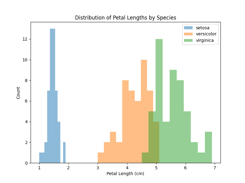
You can handle the distribution of petal lengths for different species:
1
2
3
4
5
6
7
8
9
10
11
|
plt.figure(figsize=(8, 6))
for i in range(3):
species = iris_df[iris_df['target'] == i]
plt.hist(species['petal length (cm)'], alpha=0.5, label=iris.target_names[i])
plt.xlabel('Petal Length (cm)')
plt.ylabel('Count')
plt.title('Distribution of Petal Lengths by Species')
plt.legend()
plt.show()
|
This gives us a visual overview of the differences in petal measurements between different iris species:

Application of K-Nearest Neighbors (KNN)
KNN, which stands for K-Nearest Neighbors, is a simple machine learning algorithm used for both classification and regression problems.
- Classification: To classify a data point, KNN finds the “nearest” neighbors to that point among the training data. These neighbors are determined based on the distance (e.g., Euclidean distance) from the labeled training points. The point is then classified as the majority label among its nearest neighbors (i.e., the most common class among the neighbors).
- Regression: In regression, KNN calculates the value of a point based on the values of its nearest neighbors. Typically, the value is the mean or median of the neighbor values.
KNN is useful for classification and regression problems when dealing with a limited number of features and relatively small data, especially when the relationship between features and the output label is not complex.
Import the necessary element:
1
2
3
|
from sklearn.model_selection import train_test_split
from sklearn.neighbors import KNeighborsClassifier
from sklearn.metrics import accuracy_score
|
Separate features from labels:
1
2
|
X = iris_df.drop('target', axis=1)
y = iris_df['target']
|
Split the dataset into training and test sets. Usually it is 80% and 20%, but depending on the amount and complexity of the data this setting will need to be set correctly.
Random state is a model hyperparameter used to control the randomness involved in machine learning models. In Scikit-learn, the random state hyperparameter is denoted by random_state:
1 |
X_train, X_test, y_train, y_test = train_test_split(X, y, test_size=0.2, random_state=42)
|
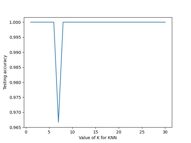
Fit method is used to train the model on training data (X_train,y_train) and predict method to do the testing on testing data (X_test). The parameter n_neighbors is the tuning parameter/hyper parameter. Choosing the optimal value of K is critical, so we fit and test the model for different values for K (from 1 to 30) using a for loop and record the KNN’s testing accuracy in a variable (scores).
1
2
3
4
5
6
7
8
9
10
11
12
13
14
15
16
17
18
19
20
21
|
k_range = range(1,31)
scores = {}
scores_list = []
# Try running from k=1 through 30 and record testing accuracy
for k in k_range:
# Initialize the KNN classifier and train it
knn = KNeighborsClassifier(n_neighbors=k)
knn.fit(X_train, y_train)
# Predict species labels for the test set
y_pred = knn.predict(X_test)
# Calculate the model's accuracy
scores[k] = metrics.accuracy_score(y_test, y_pred)
scores_list.append(metrics.accuracy_score(y_test, y_pred))
plt.plot(k_range, scores_list)
plt.xlabel("Value of K for KNN")
plt.ylabel("Testing accuracy")
|
The neighbors in KNN, in our case indicated as K, are critical because they regulate the model’s sensitivity to data details, influence the bias-variance tradeoff, and directly impact the model’s accuracy and computational requirements. Choosing an appropriate value for neighbors is essential for achieving a good balance between accuracy and the model’s ability to generalize.

For our final model we can choose a optimal value of K as 15 (which falls between 9 and 30) and retrain the model with all the available data. And that will be our final model which is ready to make predictions.
1
2
3
4
5
6
7
8
9
10
11
|
knn = KNeighborsClassifier(n_neighbors=15)
knn.fit(X_train.values, y_train.values)
x_new = [[4,3,5,2], [4,5,2,3]]
y_predict = knn.predict(x_new)
predicted_species_0 = iris.target_names[y_predict[0]]
predicted_species_1 = iris.target_names[y_predict[1]]
print(f"The predicted species for the first example data point is: {predicted_species_0}")
print(f"The predicted species for the second example data point is: {predicted_species_1}")
|
Conclusion
The Iris dataset remains a benchmark in the realms of data mining and machine learning. Leveraging Python and libraries like Pandas, Matplotlib, and Scikit-learn makes exploring and analyzing this dataset an ideal starting point for those entering the fascinating world of data mining and machine learning.
This article has provided only a glimpse into the possibilities offered by the Iris dataset and data analysis with Python. We hope it has inspired you to further explore this vast field and deepen your knowledge in data mining.
Do you need consultants or PMs for your Project in Machine Learning or Data Science? Contact us: https://www.impesud.it/contatti/ (parliamo italiano, hablamos español, speak English).


